Most lakehouse format comparisons skip the part that actually matters for streaming teams: how the format handles mutations. Apache Iceberg is excellent for append-heavy analytics, schema evolution, and multi-engine compatibility. But feed a high-churn CDC stream of updates and deletes into Iceberg using merge-on-read (MoR), and you’re managing a growing pile of delete files that accumulate between compaction runs.
Apache Paimon takes a different approach. Its Log-Structured Merge-tree (LSM-tree) architecture is designed from the ground up for continuous upserts. For the right workload (high-frequency mutations, Flink-native execution, real-time table freshness) Paimon produces a cleaner operational profile than Iceberg. For the wrong workload, it’s an unnecessary complexity burden.
The comparison also moved in 2026. Iceberg v3 replaced stacks of position delete files with deletion vectors: one compact bitmap per data file, stored in a Puffin blob, so a reader applies a single bitmap instead of opening a dozen delete files. That changes the arithmetic on the Iceberg side, and it is why this post compares three options rather than two.
This post defines the conditions where Paimon wins, where Iceberg remains the better default, and what you need to configure to use either effectively.
What Paimon Is and Where It Came From
Apache Paimon graduated to a Top-Level Project at the Apache Software Foundation in 2024 and has since progressed through several production-ready releases. It grew out of the Flink Table Store project, which explains why its design assumptions are so tightly aligned with Apache Flink.
Paimon distinguishes itself from Iceberg and Delta Lake through its choice of storage data structure. While Iceberg stores data as immutable Parquet snapshots and Hudi uses a record-level index for updates, Paimon uses an LSM-tree, the same family of data structures that underlies systems like LevelDB, RocksDB, and Apache Cassandra.
The choice of LSM-tree is not incidental. It’s a direct response to the specific access pattern of high-frequency updates.
How the LSM-Tree Handles Updates Differently
In an LSM-tree, incoming writes land in an in-memory buffer, which is periodically flushed to sorted files on disk. These sorted files are organized into levels (L0, L1, L2, and so on). Background compaction processes merge smaller files from lower levels into larger files at higher levels, resolving conflicts between earlier and later writes to the same key.
For a CDC stream where the same row might be updated many times per minute, this has concrete benefits. New CDC events always write to the in-memory buffer and are flushed to the lowest level. The query engine reads the merged view across levels. The background compaction consolidates updates at rest without blocking writes. At no point does a query need to scan separate delete files and reconcile them against data files, the LSM-tree’s merge logic handles this intrinsically.
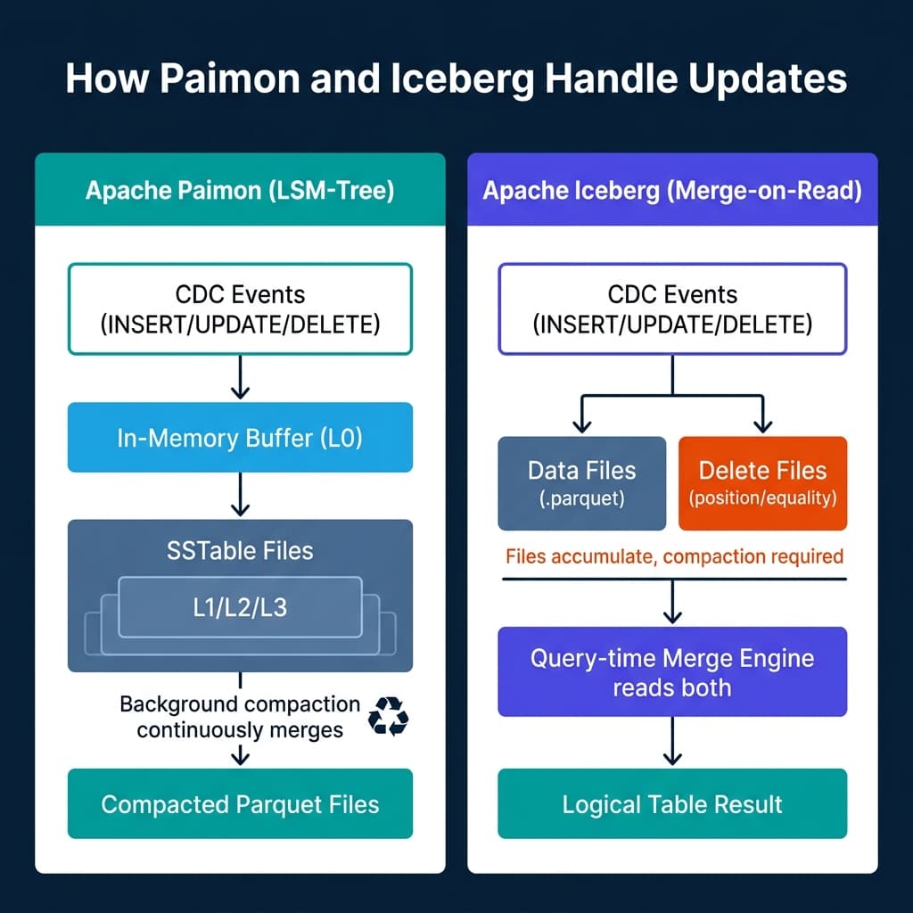
Iceberg’s approach is different. Under MoR semantics, an update to a row in Iceberg does not rewrite the data file. Instead, it writes a delete file that records the position or equality of the row to be removed, and writes a new data file containing the updated row. Queries must read both the original data files and the corresponding delete files, then apply the delete records to produce the correct result.
This works fine when updates are infrequent. When a table receives thousands of updates per second across a high-cardinality key space, delete files accumulate faster than compaction can remove them. Query performance degrades because the engine must read and reconcile more and more file pairs. The recommended remediation is more frequent compaction, which adds operational overhead and resource contention.
Paimon’s Primary Key Table: The Core Streaming Primitive
The central concept in Paimon for streaming workloads is the primary key table. When you define a table with a primary key, Paimon routes all writes for that key through the LSM-tree, resolving conflicts using the configured merge engine.
-- Create a Paimon primary key table for CDC ingestion from MySQL
CREATE TABLE customer_orders (
    order_id    BIGINT PRIMARY KEY NOT ENFORCED,
    customer_id BIGINT,
    status      STRING,
    amount      DECIMAL(10, 2),
    updated_at  TIMESTAMP(3)
) WITH (
    'connector'                 = 'paimon',
    'path'                      = 's3://data-lake/paimon/customer_orders',
    'bucket'                    = '8',
    'changelog-producer'        = 'lookup',
    'merge-engine'              = 'deduplicate'
);
The changelog-producer property controls how Paimon generates downstream changelog records for consumers of this table:
input: Assumes the input stream already contains full changelog events (+-I, -U, +U, -D). Use this when consuming from a Debezium CDC source.lookup: Generates changelogs by performing a point query on the existing table state before each write. This ensures accurate before-and-after pairs even when the input stream doesn’t carry them.full-compaction: Generates changelogs by comparing table states across full compaction cycles. Produces the most accurate changelogs but with higher latency.
The merge-engine property controls how conflicts for the same primary key are resolved. deduplicate keeps the last write. For aggregation use cases (such as a running balance or session counter) aggregation allows you to define column-level merge functions like sum, max, or last_non_null.
The Changelog Stream Feature: Why Paimon Tables Are Different from Iceberg Tables
One of Paimon’s most distinctive capabilities is that primary key tables can serve as both a batch-readable lakehouse table and a changelog source for downstream Flink jobs.
When a Flink job reads a Paimon primary key table as a streaming source, it doesn’t read static snapshots. It reads the changelog stream, a continuous stream of +I, -U, +U, and -D records that represent every mutation to the table. This means you can chain Flink jobs where the output of one job becomes the changelog input of the next, building multi-stage stateful streaming pipelines that maintain real-time derived tables.
Iceberg can serve as a streaming source in Flink through incremental reads, but its model is snapshot-based. Flink reads successive Iceberg snapshots and emits new or deleted rows detected between them. This works for append-only tables and bounded update patterns, but doesn’t produce the full changelog semantics that Paimon emits natively. Building an accurate changelog from Iceberg incremental reads requires additional logic to handle updates that touch the same row across multiple snapshots.
Where Paimon Falls Short
Paimon’s ecosystem reach is its most significant constraint. As of mid-2025, the query engines with strong Paimon read support are Apache Flink and Apache Spark. Trino has a community-maintained Paimon connector, but it lacks some of the more advanced Paimon table features. Engines like Dremio, DuckDB, and Snowflake don’t have native Paimon integration.
If your architecture requires ad-hoc SQL from multiple query engines, particularly BI tools that connect through Trino or Presto, Iceberg’s ecosystem compatibility is a clear advantage. Nearly every modern query engine supports Iceberg out of the box.
Paimon does offer an Iceberg-compatible read path, which exposes Paimon tables as Iceberg tables to engines that support the Iceberg REST Catalog API. This compatibility layer allows engines like Spark and Trino to read Paimon data without native Paimon support. However, the compatibility layer is read-only and doesn’t expose Paimon’s changelog semantics. You get table data but not the streaming mutation stream.
Another constraint is operational maturity. Iceberg has a larger user base, more documented failure patterns, and more tooling for maintenance, governance, and catalog integration. Teams evaluating Paimon for production use should plan for less community documentation on edge cases and a steeper learning curve on tuning the LSM-tree parameters.
How Iceberg v3 Deletion Vectors Change the Comparison
For most of Iceberg’s history, the cost of a merge-on-read update was paid at read time. A commit that deleted 400 rows across 40 data files wrote delete records into Parquet delete files, each tagged with the data file it applied to. Every later read of those files had to open the deletes, decode the positions, and filter rows. After a few hundred commits, one data file might be covered by a dozen delete files, most of them superseded by later ones.
Iceberg v3 introduced deletion vectors. A deletion vector is a bitmap with one bit per row position in a single data file, stored as a blob inside a Puffin file. Each data file has at most one active deletion vector, and a commit that deletes more rows in that file merges the new positions into the existing bitmap instead of adding another file to a stack.
The specification details and merge semantics are covered in How Iceberg V3 Deletion Vectors Fixed Merge-on-Read for Streaming Tables. What matters for this comparison is what the change does to three costs.
Metadata growth stops compounding. Under v2, delete metadata per data file grew with the number of commits that touched it. Under v3 it grows with the row count of the data file, because the bitmap is one bit per row. A 100,000-row data file has a deletion vector of at most 12.5 KB before compression, whether the deletions arrived in one commit or two hundred. A delete-heavy table’s manifest list stops accumulating references to hundreds of small delete files, and planning time stops degrading as a function of commit history.
Reader work drops to a bitmap check. A v3 reader opens the data file, loads one Puffin blob, and tests bits as it scans row groups. There is no delete file to join and no position set to materialize, and an engine can skip a row group whose bits are all set without decoding it.
One thing does not change. Deleted rows are still physically present. A deletion vector marks rows dead, it does not remove bytes from Parquet or reduce scan I/O where a row group mixes live and deleted rows. A table that deletes 60 percent of its rows still reads 100 percent of its bytes until compaction rewrites the file. Space amplification, and the rewrite job that fixes it, survive into v3. What v3 removes is write amplification of delete metadata and read amplification from stacked delete files.
That rebalances which side carries the burden. Under v2, high churn caused two failures at once: delete files piled up until reads slowed, and compaction had to merge delete files as well as rewrite data. Under v3 the first is gone, so a job committing every few seconds sees flat per-file metadata and stable read latency between compactions. The second remains: compaction still rewrites data files to reclaim space, and file count still grows with write volume. Paimon keeps that count bounded by bucket count and level configuration, an engine invariant rather than a maintenance decision.
Reading current state differs too. A Paimon point lookup for one key goes through the LSM index into one bucket, touching a bounded number of sorted runs with bloom filters. An Iceberg v3 point lookup prunes manifests to candidate files, reads them, and applies any deletion vector attached to each. Deletion vectors made that cheaper but did not give Iceberg a primary key index, so the reader still finds a row before deciding it is dead. An LSM-tree can reject a file without reading it.
Two consequences follow. First, the churn level where Iceberg v3 becomes painful is higher than for v2 but still exists, and it is measured in data files rather than delete files. A table taking 5,000 updates per second into 128 MB files produces a new file every few seconds, tens of thousands per day before compaction. Deletion vectors hold the delete side flat. They do not reduce file count, so the scheduling burden shifts to compaction and snapshot expiration.
Second, deletion vectors do not give streaming teams a changelog. They tell a reader which rows are dead, not what a row looked like before an update. That is row lineage in v3, a separate mechanism with its own adoption curve. Paimon solves the same problem inside the format with input, lookup, and full-compaction producers, which is why its pipelines chain jobs without external state. Iceberg v3 can produce a changelog from an incremental scan between snapshots, but pairing before and after images depends on row lineage and reader support.
So the 2026 framing is narrower than the 2024 one. Paimon’s advantage is no longer that Iceberg falls over under updates. It is that Paimon treats continuous mutation as the normal case, with an index, bounded file counts, and a native changelog, while Iceberg v3 treats it as a supported case with cheap delete metadata and a maintenance schedule attached. A steady stream plus disciplined maintenance closes most of the gap. A bursty stream, high-cardinality keys, and jobs that need changelog records from the table keep it wide.
Write Path, Read Path, Compaction: Side by Side
Trace one upsert through each format and count what lands on storage, what the reader does, and what work is owed afterward.
| Stage | Paimon primary key table | Iceberg v2 merge-on-read | Iceberg v3 with deletion vectors |
|---|---|---|---|
| What an upsert writes | A row appended to the in-memory buffer, flushed as a sorted run at L0 in the target bucket. One commit writes one new file plus manifest updates. | A Parquet data file with the new row version, a position delete file (or equality delete file) marking the old row, and updated manifests in a new snapshot. | A Parquet data file with the new row version, a merged Puffin deletion vector for each affected data file, and updated manifests in a new snapshot. |
| What a reader merges at query time | Sorted runs across levels within each bucket, resolved by primary key with the configured merge engine. Bloom filters skip runs that cannot hold a key. | Data files plus every delete file referencing them, decoded into a position set and applied row by row. Cost grows with delete files per data file. | Data files plus at most one Puffin bitmap per data file, tested per row position. Cost is constant per file regardless of commit count. |
| What background compaction does | Merges L0 sorted runs into higher levels, resolving duplicate keys and dropping superseded versions. Bounded work per bucket, triggered by sorted run count. | Merges delete files and rewrites data files to drop deleted rows. Two jobs, and delete file merging is often the more urgent one. | Rewrites data files to drop deleted rows and discard their deletion vectors. One job, driven by the deleted-row ratio per file. |
| How changelog consumers read changes | Natively, through changelog-producer modes emitting +I, -U, +U, -D records as a Flink source, with no external state. | Incremental scan between two snapshots, emitting inserted and deleted rows. Reconstructing before and after values for a key is application logic. | Incremental scan between two snapshots, with row lineage fields (_row, _last_updated_sequence_number) available for pairing versions when enabled and supported. |
Three things fall out of that table.
The write path favors Paimon on volume and Iceberg on predictability. A Paimon commit is small in bytes because it appends a sorted run and updates manifests, and the LSM-tree amortizes merging across levels. An Iceberg commit materializes full Parquet files for new row versions, so a stream updating 100 rows per second with 5-second commits writes 500 rows of new files per commit and leaves old versions on disk until compaction. Deletion vectors shrink the delete side of that write, not the data side.
The read path is where v3 closed most of the distance. Under v2, read cost per data file scaled with delete file count, so an updated table got slower through the day and faster after maintenance. Under v3 it is a bitmap test that stays flat between compactions, and Paimon’s read cost tracks sorted run count per bucket, also bounded. Both formats now degrade with maintenance lag rather than with update count.
Compaction is where the operational difference lives. Paimon compaction is internal: the engine merges L0 runs when a threshold is crossed, and no separate delete merge needs scheduling. Iceberg compaction is an explicit job with a target file size and a rewrite threshold, owned by the team. Deletion vectors cut the jobs from two to one, a real reduction in toil, but the remaining job is still mandatory. A v3 table with continuous deletes and no compaction accumulates dead bytes.
The changelog row is the least symmetric. Paimon’s changelog is an output of the table format, configured at create time, with an explicit accuracy-versus-latency tradeoff. Iceberg’s is a scan pattern over snapshots, and before-and-after pairs depend on row lineage plus reader support. If each pipeline stage needs the previous stage’s full change stream, that asymmetry outweighs any difference in write or read cost.
No benchmark numbers appear here, deliberately. Throughput depends on file sizing, bucket counts, commit intervals, engine versions, and object store behavior, and published comparisons rarely hold those constant. Run both against your own event rate.
The Workload Decision Matrix
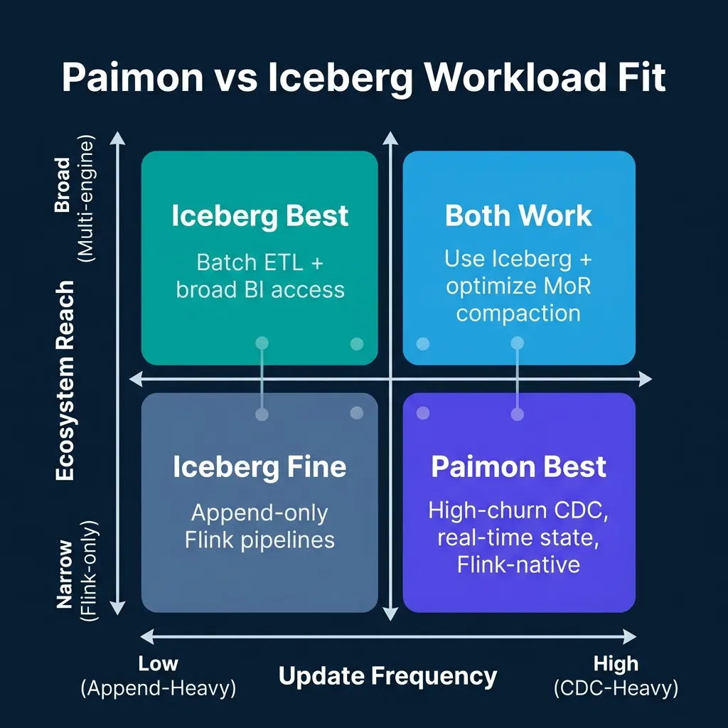
The decision narrows to two dimensions: how frequently your tables receive updates and how many engines need to read the data. Iceberg v3 splits the second dimension, because a table with deletion vectors is still a standard Iceberg table that every Iceberg reader can open, while its behavior under churn differs sharply from v2.
| Criterion | Paimon primary key table | Iceberg v2 merge-on-read | Iceberg v3 with deletion vectors |
|---|---|---|---|
| Sustained high churn (thousands of updates per second, high-cardinality keys) | Designed case. Churn becomes sorted runs, file count bounded by buckets and levels. | Weakest case. Delete files accumulate per file, reads degrade with commit history. | Workable. Delete metadata stays flat per file, but file count and rewrite load grow with write volume. |
| Moderate churn with batch analytics on the same table | Works, at the cost of a second format and a second compaction model. | Acceptable with a scheduled rewrite job. | Best fit. Flat delete metadata plus one rewrite job. |
| Append-heavy ingestion, occasional late updates | Overkill. LSM machinery for a table that barely mutates. | Fine, and no reason to choose merge-on-read. | Fine, and no reason to choose merge-on-read. |
| Multi-engine and BI access | Flink and Spark native, Trino partial, no Dremio, DuckDB, or Snowflake. | Broad, though each reader must implement the delete spec. | Broad, and v3-aware readers avoid delete file stacking. Verify engine support for v3 and Puffin before committing. |
| Native changelog for downstream jobs | Yes, with input, lookup, and full-compaction producers. | No. Incremental scan plus application logic. | Partial. Incremental scan plus row lineage, where reader support exists. |
| Operational burden | Tune buckets, compaction trigger, full-compaction interval, in less documented territory. | Two jobs: delete file merge and data file rewrite. | One job: data file rewrite. More tooling and documentation than Paimon. |
Read down the columns and the verdicts land where the workloads suggest.
High-frequency CDC, Flink-native execution, real-time freshness: Paimon’s optimal case. Orders that update dozens of times per lifecycle, inventory with near-continuous SKU updates, session tables that change several times per minute. Deletion vectors do not change this verdict, because the binding constraint is a changelog for downstream Flink jobs and an index for point lookups.
High-frequency CDC, multi-engine reads, no Flink dependency: The case v3 changed. Continuous updates read by Spark, Trino, and a warehouse connector no longer force a choice between delete file accumulation and a second format. Turn on deletion vectors, keep files large enough that a rewrite has work per file, and compact on the deleted-row ratio. The catch is engine support: a v3 table is only as good as the slowest reader in your fleet.
Batch ETL with broad BI access: Iceberg wins without competition. Appending daily partitions and querying from Trino, Dremio, Snowflake, and Spark comes down to multi-engine support and governance maturity. Deletion vectors are irrelevant to a table that only appends.
Mixed workload, moderate update frequency: Both work. With existing Iceberg infrastructure, tuning compaction and using copy-on-write (CoW) for large-batch updates is simpler than adding a second format. Where updates are frequent but commits are small, v3 merge-on-read with deletion vectors is a defensible default. Adopt Paimon selectively for the tables where it demonstrably helps.
Practical Configuration for High-Churn Paimon Tables
When tuning a Paimon primary key table for a high-churn CDC source, three settings matter most.
Bucket count: Paimon distributes data by primary key across a fixed number of buckets. Each bucket holds an LSM-tree. More buckets allow more write parallelism but increase the number of small files at low data volumes. For a table with millions of rows and hundreds of thousands of updates per minute, 16 to 64 buckets is a reasonable starting range.
Compaction trigger: Paimon triggers compaction when the number of sorted files at level 0 exceeds a threshold. The default threshold is 5. For very high write rates, reducing this to 3 keeps the LSM-tree shallow and maintains consistent read performance. For lower write rates, increasing the threshold to 8 or 10 reduces compaction frequency and I/O overhead.
Full-compaction interval: For tables serving changelog consumers, schedule periodic full compaction to ensure that changelog events are complete and accurate. Lookup-mode changelog producers generate accurate changelogs on individual writes, but full compaction provides a consistency checkpoint that catches any drift between levels.
-- Configure a high-churn Paimon table with aggressive compaction settings
ALTER TABLE customer_orders SET (
    'num-sorted-run.compaction-trigger' = '3',
    'full-compaction.delta-commits'     = '20',
    'write.merge-engine'                = 'deduplicate'
);
Paimon Tags: Batch-Compatible Snapshots for CDC Tables
One of Paimon’s useful operational features is the Tag system. Unlike Iceberg’s snapshot-based time travel (which is tied to all historical snapshots), Paimon Tags allow you to mark specific points in a table’s history for long-term retention.
Tags are particularly valuable for CDC tables where you want to support both the streaming changelog use case and the batch analytics use case simultaneously:
-- Create a daily tag for batch processing access
CALL sys.create_tag('my_catalog.default.customer_orders', '2025-05-24', 2 /*snapshot-id*/);

-- Read from a tagged version for batch analytics
SELECT * FROM customer_orders /*+ OPTIONS('scan.tag-name'='2025-05-24') */;

-- Expire snapshots while retaining tags
CALL sys.expire_snapshots('my_catalog.default.customer_orders', '2025-05-24 00:00:00', 10 /*retain-latest*/);
Tags persist independently from snapshots. You can expire Paimon snapshots aggressively to control storage costs while retaining daily or weekly tags for historical analytical access. This gives CDC tables the same time-travel capability that makes Iceberg valuable for audit use cases, without the storage cost of retaining every intermediate snapshot.
Streaming Aggregations with Paimon’s Aggregation Merge Engine
One of Paimon’s most distinctive features is its native support for streaming aggregations, running computations that accumulate over time directly in the table format.
The aggregation merge engine allows defining column-level merge functions that resolve conflicts for the same primary key:
-- Paimon table for session-level aggregations
CREATE TABLE user_sessions (
    user_id             BIGINT PRIMARY KEY NOT ENFORCED,
    session_count       INT,
    total_purchase_amt  DOUBLE,
    last_active         TIMESTAMP(3),
    active_days         BIGINT
) WITH (
    'connector'     = 'paimon',
    'path'          = 's3://data-lake/paimon/user_sessions',
    'merge-engine'  = 'aggregation',
    'fields.session_count.aggregate-function'         = 'sum',
    'fields.total_purchase_amt.aggregate-function'    = 'sum',
    'fields.last_active.aggregate-function'           = 'last_non_null',
    'fields.active_days.aggregate-function'           = 'count'
);
Incoming events contain partial updates: a new session event increments session_count by 1, adds the purchase amount to total_purchase_amt, and updates last_active to the event timestamp. Paimon’s LSM-tree merge logic applies these aggregations at compaction time, accumulating the correct running totals without requiring a stateful Flink operator to maintain the aggregation in RocksDB.
This pattern is particularly efficient for analytics tables that are updated continuously from streaming sources but queried on a batch schedule. The aggregation merge engine handles the incremental state in the table format itself, rather than requiring complex stateful stream processing.
Monitoring Paimon Tables in Production
Paimon doesn’t have the same ecosystem of monitoring tooling as Iceberg (which benefits from tools like PyIceberg’s table introspection and Spark’s DESCRIBE HISTORY). But Paimon exposes sufficient system tables for building operational monitoring:
-- Check LSM-tree file count across buckets
SELECT bucket, level, count(*) as file_count
FROM customer_orders$files
GROUP BY bucket, level
ORDER BY bucket, level;

-- Check snapshot history
SELECT snapshot_id, schema_id, commit_time, total-size
FROM customer_orders$snapshots
ORDER BY commit_time DESC
LIMIT 20;
Metrics to watch in production Paimon environments:
- L0 file count per bucket: High L0 file counts (>5) indicate compaction is falling behind write throughput. This degrades read performance as the query engine must merge more sorted runs.
- Compaction lag time: How recently did the last full compaction complete? For changelog-producing tables, stale compaction creates gaps in downstream changelog accuracy.
- Storage size per bucket: Uneven distribution across buckets indicates poor key distribution. Hot buckets receive disproportionate writes and compact more frequently than cold buckets, creating performance inconsistency.
Paimon’s Flink integration also exposes JVM metrics for compaction thread pool saturation, which can be monitored through Prometheus/Grafana for operational alerting.
Running Both: Paimon for the Hot Stream, Iceberg for the Table of Record
You do not have to choose one format for an entire platform. A pattern that has settled into practice keeps Paimon as the ingestion surface for high-churn streams and Iceberg as the table of record that every engine reads.
CDC events from Debezium or a Flink CDC connector land in a Paimon primary key table, which absorbs the churn, serves point lookups to Flink jobs, and emits a changelog to downstream streaming stages. On a schedule, a batch job reads a Paimon tag, a stable snapshot at a known point, and writes it into an Iceberg table as an append or a merge against the previous export. Everything downstream of Iceberg, meaning Trino, Dremio, Snowflake, Spark, and the BI tools pointed at them, reads the Iceberg copy and never touches Paimon.
The scheduling choice is the interesting part. A daily tag is simple and cheap, and the Iceberg table lags the streaming table by up to a day. An hourly export keeps lag small at the cost of an hourly read plus write, fine for millions of rows and less fine for billions. The export can also be incremental: read the tag, compare against the last exported tag using row lineage fields where enabled, and merge only changed rows. That is more engineering than most teams need on day one.
What this buys is the ecosystem problem solved without giving up churn handling. Paimon’s weakness was never storage efficiency or write throughput, it was that analysts on Trino and Dremio could not query it well. A readable Iceberg copy removes that constraint and picks up v3 features on its own.
What it costs is a second format and a batch job: two compaction models, two monitoring setups, two catalogs, and a consistency question whenever someone asks why the tables disagree. The answer is usually that the export has not run yet, so put a freshness timestamp on the Iceberg table that consumers can check.
Three conditions make the overhead worth it. The stream is genuinely high-churn, meaning updates to the same keys arrive continuously. A real population of readers sits outside Flink and Spark. And their freshness requirement is coarser than the streaming consumers’, so an hourly or daily copy is acceptable. If external readers need second-level freshness, the export becomes a replication pipeline, and the better question is whether they can read Paimon through its Iceberg-compatible read path.
Two related posts cover the design questions. What Iceberg V3 Advances Mean for CDC Pipelines covers how v3 changes what a CDC pipeline can push into the table layer. Iceberg Row Lineage: The Feature AI and CDC Workloads Will Eventually Depend On covers the identity mechanism behind incremental export. Both matter at the export step, because row lineage is what lets a batch job identify changed rows between two tags instead of comparing full snapshots.
Conclusion
Paimon is not a general-purpose Iceberg replacement. It’s a purpose-built tool for a specific problem: high-frequency mutations in streaming lakehouse architectures, particularly where Apache Flink is the primary compute engine and real-time table freshness is a hard requirement.
Iceberg v3 narrowed that problem without erasing it. Deletion vectors replaced stacks of position delete files with one bitmap per data file, removing the failure mode where read latency drifted up with commit history. They did not remove the physical rewrite of data files, the file growth that tracks write volume, or the absence of a native changelog and a primary key index. Those are why a high-churn Flink pipeline still belongs on Paimon.
For append-heavy pipelines, mixed-engine analytics, or organizations already invested in Iceberg governance tooling, Iceberg remains the better default, and on v3 it is a better default than it was. The format choice should follow the workload, not the other way around.
The clearest signal that Paimon is worth evaluating is mounting operational complexity around Iceberg compaction on high-churn tables. If you spend more time managing file accumulation and compaction schedules than building pipeline features, and downstream jobs need a changelog the format cannot emit, test Paimon’s LSM-tree model against your throughput numbers. If the complexity is real but the changelog requirement is not, Iceberg v3 with deletion vectors and a disciplined rewrite schedule is the cheaper answer.
Go Further with Lakehouse Architecture
For a comprehensive guide to modern data architectures including open table format comparisons, streaming lakehouse design, and AI-native data platforms, pick up The 2026 Guide to Lakehouses, Apache Iceberg and Agentic AI: A Hands-On Practitioner’s Guide to Modern Data Architecture, Open Table Formats, and Agentic AI.
Browse Alex’s other data engineering and analytics books at books.alexmerced.com.
To query both Paimon and Iceberg tables with unified sub-second performance and automated reflection caching, try Dremio Cloud free at dremio.com/get-started.